
Machine learning challenges in production: causes and fixes

Contents
Machine learning projects rarely fail on the algorithm. They fail where data, deployment and ownership meet, and the order of the failure matters: a drifting model, a skewed feature pipeline and a biased training set look alike in a dashboard but need different fixes.
The challenges below follow the lifecycle (data, model, deployment, operations) so a team with a failing model can work from the cheapest checks to the most expensive. How much each one hurts depends on your label delay, regulatory exposure and who owns the model after launch.
Machine learning challenges in production, in diagnostic order
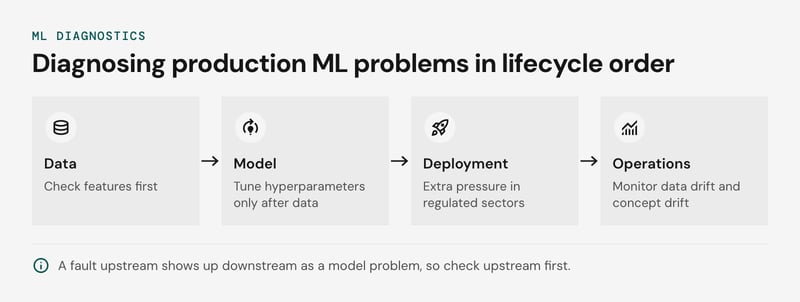
Machine learning challenges in production are best diagnosed in lifecycle order: data, model, deployment, operations. A fault upstream shows up downstream as a model problem, so tuning hyperparameters before checking features wastes effort. Teams in regulated sectors face extra pressure on compliance and deployment, which is why MLOps in financial services is a useful reference for structuring these checks.
Netguru designs and builds machine learning products and the MLOps pipelines behind them. We recommend wiring model monitoring for data drift and concept drift before launch, because ownership is easiest to assign while the pipeline is still being built.
For a model already live, start at operations instead, since late-arriving labels hide concept drift the longest. If you need a partner to build and operate these pipelines, Netguru's AI development services cover the full lifecycle from data to deployment.
How does poor data quality break ML projects?
Poor data quality breaks ML projects by letting a model score well on the wrong metric, and class imbalance in fraud detection shows how.
Assume a stream of 100,000 transactions in which 100 are fraudulent. These figures are illustrative, not a benchmark. Two models give very different pictures depending on the metric:
| Model | Flagged | Fraud caught | Accuracy | Precision | Recall |
|---|---|---|---|---|---|
| Always predicts "legitimate" | 0 | 0 | 99.9% | undefined | 0% |
| Trained classifier | 150 | 60 | 99.87% | 40% | 60% |
The majority-class model wins on accuracy and catches no fraud. Under this imbalance, accuracy cannot separate a useful fraud model from a useless one. Evaluate with the precision-recall curve and PR AUC, then choose the threshold from the cost of an analyst review against the cost of a missed fraud. ROC AUC can also look flattering at this skew.
Two fixes dominate, class weights and SMOTE, and each has a price; the next section compares them. Whichever you choose, recalibrate before treating scores as risk estimates.
Algorithmic bias enters through the same door. If fraud labels come from past investigator decisions, or one customer segment is thinly sampled, the model reproduces those gaps. Report precision and recall per segment, not only in aggregate.
Class imbalance and labeling problems: Class weights or SMOTE?
Use class weights first for class imbalance, and add SMOTE only when the minority class is too sparse for the model to learn from.
Class weights (class_weight="balanced" in scikit-learn) leave the rows untouched and reweight the loss, so nothing can leak between folds. The cost is calibration: predicted probabilities for the minority class inflate. Recalibrate with isotonic or Platt scaling on an untouched validation set, or choose the decision threshold from the precision-recall curve.
SMOTE interpolates synthetic minority rows between nearest neighbors. If you apply it before the split, synthetic points built from validation-fold neighbors leak into training, and offline scores overstate production performance. Put the sampler inside imbalanced-learn's Pipeline, which resamples only during fit. SMOTE also tends to overfit noisy minority regions.
Check label quality before choosing either. Have two annotators label a shared sample and compute Cohen's kappa per class (Krippendorff's alpha for more than two annotators). Low agreement on the minority class means SMOTE interpolates between mislabeled points and class weights increase the noise, so fix the labeling guideline first.
Overfitting and underfitting: How to spot and fix them
Overfitting shows up as a wide gap between training and validation scores, and underfitting shows up as both scores being poor. Read the gap first, then pick the fix.
A network can memorize the training set, score 100 percent accuracy on it, and still fail on new data. A learning curve, with both scores plotted against training set size, separates the cases:
| Symptom | Diagnosis | First fix | Trade-off |
|---|---|---|---|
| High train score, low validation score | Overfitting | L2 or dropout, early stopping, shallower trees | Adds bias; strength needs tuning |
| Both scores low and flat | Underfitting | More features, higher capacity, weaker regularization | Variance rises again |
| Gap narrows as data grows | Data-limited | More data or augmentation | Labeling cost |
| Validation score swings between folds | High variance estimate | Stratified k-fold | k times the compute |
For time-ordered data, use time-based splits, because shuffled k-fold leaks future rows into training.
Log every run in MLflow so each fix is comparable. Record hyperparameters, the git commit, a dataset version from DVC, and train and validation metrics per epoch.
Without experiment tracking you cannot tell whether a better validation score came from regularization or from a changed split. MLflow, the open source platform whose Tracking component logs experiments, gets over 30 million package downloads a month (MLflow (mlflow.org), 2025).
Repeated tuning against one validation set overfits that set too. Keep a test set and score it once, after the last run.
Why is model interpretability hard to deliver?
Model interpretability is hard because accurate models spread each prediction across thousands of interacting parameters, so SHAP and LIME can only approximate the reasoning after the fact.
Opacity blocks adoption where decisions must be contested or verified. A credit applicant cannot appeal a denial nobody can explain, a clinician cannot check a prediction against physiology, and a driverless-car team cannot trace a perception failure to its cause. Interpretability is also a debugging tool: attributions expose leaked features and spurious correlations before users do.
The two common post-hoc methods trade cost against stability:
| Criterion | SHAP | LIME |
|---|---|---|
| Cost per prediction | Low for tree ensembles with TreeExplainer, high for KernelSHAP on wide inputs | Low, one local surrogate fit |
| Stability | Consistent attributions grounded in Shapley values | Varies with perturbation sampling and kernel width |
| Scope | Local and global | Local only |
| Best use | Audits, model reviews, regulated decisions | Fast spot checks on text and image models |
We recommend SHAP wherever the model is a tree ensemble, because exact attributions come cheaply. For deep networks and large inputs, use LIME for triage, fix the random seed, and rerun each explanation several times. If the top features change between runs, do not trust that explanation.
Both methods explain the model, not the world. Correlated features split credit unpredictably, and an attribution says nothing about causation. For automated decisions, Article 13(2)(f) GDPR requires "meaningful information about the logic involved". Whether feature attributions meet that standard is a question for legal counsel.
Where does bias in ML models come from?
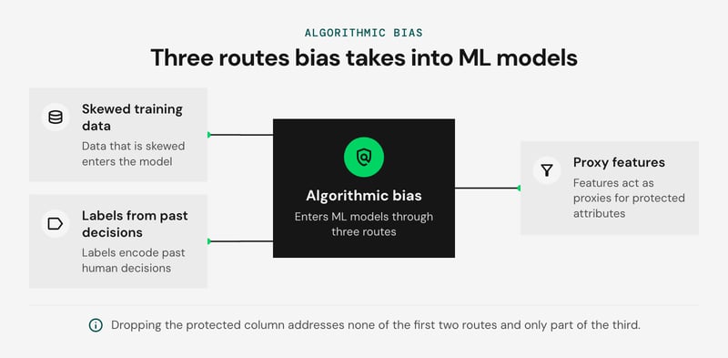
Algorithmic bias in ML models enters through three routes: skewed training data, labels that encode past human decisions, and features that act as proxies for protected attributes. Dropping the protected column addresses none of the first two and only part of the third.
Take an illustrative hiring model trained on historical recruiter decisions, with gender removed from the features. Assume the company hired mostly men for engineering roles. The labels carry that history, and features such as previous employer, university society, or employment gaps correlate with gender, so the model reconstructs it.
A subgroup audit catches this before launch. Keep gender in the evaluation set only, then compare selection rate and true positive rate per group, for example with Fairlearn's MetricFrame. A large gap among equally qualified candidates blocks the release.
SHAP attributions then show which features carry the gap, which is where model interpretability earns its cost, although it shows that the model uses a proxy, not why the proxy correlates with gender.
Removing the proxy often shifts weight to the next most correlated feature, so re-run the audit after each change. Reweighing and fairness constraints trade some overall accuracy for smaller gaps. How much accuracy to give up is a product and legal decision.
Credit scoring follows the same pattern. Postal code can stand in for ethnicity, and labels exist only for applicants who were approved before, so the model never sees outcomes for the people it would have rejected.
Auditing needs protected-attribute data. Article 4a(1) of the AI Act lets providers of high-risk systems process special categories for bias detection only where strictly necessary, with safeguards including deletion once the bias is corrected. Confirm your lawful basis with legal counsel.
Why do ML models fail between prototype and production?
ML models fail between prototype and production mostly because the serving path computes features differently from the training path, and because legacy systems impose input formats and latency budgets the notebook never faced.
Training-serving skew is the common form. A pandas transformation from training gets rewritten in Java or SQL for the service, and null handling, rounding, or time windows drift apart. MLOps pipelines exist to remove that divergence by sharing one feature definition across both paths. Google's Rules of Machine Learning (Rule 29) advises logging the features used at serving time and reusing them for training.
Legacy integration adds batch-only data feeds, undocumented schemas, and synchronous calls with strict timeouts. Sculley et al. (NeurIPS 2015) identify glue code around the model as a main source of hidden technical debt. Keeping that glue code and the legacy systems around it healthy is an ongoing task, which is why many teams pair their ML work with dedicated enterprise software maintenance.
Skew produces the same symptom as overfitting, a model that scores well offline and fails on live data, from a different cause. Offline evaluation cannot separate the two because it reads features from the training pipeline.
Shadow deployment sends a copy of live production requests to the candidate model and logs its predictions without returning them to users. Comparing the logged serving features against training features, and the candidate's score distribution against the incumbent's, surfaces skew, schema breaks, and latency problems that a held-out test set cannot show, with no user risk.
The three rollout strategies catch different failures:
| Strategy | Traffic and exposure | Catches | Misses |
|---|---|---|---|
| Shadow | Mirrored requests, outputs logged and never served | Training-serving skew, schema and feature errors, latency under real load, score distribution shifts | User response to predictions, feedback effects |
| Canary | Small share of real users gets the new model | Business-metric regressions, error rates, real user behavior | Problems in rare segments if the slice is small; exposes some users to errors |
| Blue-green | Two full environments, traffic switched at once | Infrastructure and configuration faults, with instant rollback | Model quality problems before the switch |
We recommend running them in sequence: shadow first, then canary, then blue-green for the final switch and rollback. MLflow's model registry pins which model version sits in shadow, and DVC versions the training data that the feature baselines come from, so the comparison is reproducible.
Shadow mode doubles inference cost for the test period. It also cannot cover models whose predictions trigger side effects such as payments. Those models go to a narrow canary behind a feature flag.
How to detect model drift in production after launch
Detect model drift after launch by monitoring input distributions with the population stability index or a Kolmogorov-Smirnov test first, because labels arrive too late for accuracy to raise the first alarm.
The order of signals follows label delay. Assume a credit model whose outcomes land 45 days after scoring (an illustrative figure). Accuracy then describes the model as it was six weeks ago, so model monitoring has to start from signals that need no ground truth.
The signals side by side:
| Signal | Needs labels | What it catches | When it fires |
|---|---|---|---|
| PSI or KS test on input features | No | Data drift | Days |
| Prediction score distribution | No | Data drift and some concept drift | Days |
| Proxy outcomes (early repayment, click-through) | Partly | Early concept drift | Days to weeks |
| Accuracy, recall, calibration | Yes | Concept drift | After the label delay |
PSI compares binned distributions of a production window against a training or reference window, and the bin edges you choose change the score. The KS test compares empirical distributions without binning, but on large windows it flags shifts too small to matter.
Evidently AI supports both as selectable drift tests, with defaults that vary with sample size and feature type (open-source drift detection tools review, arXiv).
Data drift and concept drift need different handling. Input tests see data drift, a change in the feature distribution. Concept drift is a change in the relationship between features and the target, and it can occur with every input distribution unchanged. Only labels or a proxy outcome expose it, so a quiet PSI dashboard does not prove the model is healthy.
Our recommended retraining rule has two triggers, and whichever fires first starts a retrain:
- Drift threshold: PSI or KS flags the features that carry most of the model's importance (rank them by SHAP) in several consecutive windows. A single-window spike is often a seasonal or upstream pipeline artifact.
- Calendar floor: retrain on a fixed cadence, such as quarterly (an illustrative interval), even when no alarm fires. This covers the concept drift that input tests cannot see.
A common convention treats PSI above 0.25 as a major shift, but that cutoff is a rule of thumb, so calibrate it against your own history.
Gate every retrained candidate behind a shadow deployment, and promote it only after labels that have since landed confirm it beats the incumbent. Where labels arrive within hours, as in ad ranking, skip the proxy layer and alert on accuracy directly. Input tests then help diagnose why accuracy moved.
How privacy, security and regulation constrain ML
Privacy, security, and regulation constrain ML by dictating what training data you may keep, what the model may reveal, and what evidence the retraining pipeline must produce. Treat them as MLOps requirements, because each one maps to a pipeline stage.
Under Regulation (EU) 2024/1689, Article 113 sets general application from 2 August 2026. Annex III high-risk systems follow from 2 December 2027 under Article 113(c)(i). Credit scoring is generally treated as an Annex III use case, but counsel should confirm whether your model is in scope.
The mapping for a retraining pipeline:
| Stage | Provision | Control |
|---|---|---|
| Ingestion | GDPR Article 32(1)(a) | Pseudonymize at the boundary. |
| Bias testing | AI Act Article 4a(1) | Keep special-category attributes in a separate, access-logged store. Delete them once the bias is corrected, per Article 4a(1)(e). |
| Evaluation | AI Act Article 15(3) | Declared accuracy metrics go in the model registry next to the artifact. |
| Continuous learning | AI Act Article 15(4) | Break feedback loops, so biased outputs do not feed the next training set. |
| Serving | GDPR Articles 13(2)(f) and 22 | Provide a human-review path and SHAP reason codes for automated decisions. |
SHAP reason codes cost compute at serving time, so batch them for declined applications. Model interpretability then supports the Article 13(2)(f) duty to give meaningful information about the logic involved.
Membership inference is the attack that retraining makes worse. Each retrain on fresh records exposes another snapshot, and overfit models tend to separate training members from non-members by prediction confidence.
The mitigations carry trade-offs:
- Early stopping and regularization: cheap, but they only reduce leakage.
- Returning labels instead of scores: removes the confidence signal, but breaks downstream threshold tuning.
- DP-SGD: gives a formal privacy bound, at a cost in accuracy and training time that grows as the privacy budget tightens.
Run the same attack against each retrained candidate before promotion, and treat a failing audit as a blocked release.
What drives the cost of ML in production?
Post-launch ML cost comes mostly from recurring compute and people: retraining cadence, GPU hours per run, MLOps tooling, and who is on call for the model.
Sculley et al. argue in Hidden Technical Debt in Machine Learning Systems that ML systems carry ongoing maintenance costs that are easy to miss at launch. The trade-offs behind those costs are why some teams choose to outsource machine learning maintenance and operations to an external partner.
| Driver | What scales it | Trade-off |
|---|---|---|
| Retraining cadence | Drift speed, label latency | Frequent retrains cut stale-model risk but multiply GPU hours and validation work. Drift-triggered runs on top of a slow schedule usually cost less (our judgement) |
| GPU hours per run | Model size, data volume, hyperparameter search | Fine-tuning or warm starts are cheaper per run, but errors can accumulate until a full retrain |
| Model monitoring and experiment tracking | Metric count, run history, storage | Self-hosted MLflow and Evidently AI avoid license fees and cost engineer time. Managed platforms reverse that |
| On-call ownership | Alert volume, model criticality | Rotations cost salary time but shorten time to rollback |
A part-time data scientist owning a production model is the riskiest staffing pattern. Alerts wait for sprint capacity, retraining lives in notebooks, and the cost surfaces later as an outage or silent accuracy loss.
We recommend a named owner with an on-call rotation and a platform engineer for pipelines, even at fractional allocation. A single low-stakes batch model may not need that.
Machine learning challenges and mitigations at a glance
Machine learning challenges tend to surface in a fixed order: class imbalance at data preparation, overfitting at training, algorithmic bias at evaluation, and concept drift once model monitoring is live. A skills gap runs under all of it. We suggest diagnosing in that order, because a later symptom is often caused by an earlier stage.
The table maps each symptom to the cheapest first check:
| Stage | Symptom | First check | Fix |
|---|---|---|---|
| Data preparation | High accuracy, poor minority-class recall | Per-class confusion matrix; label agreement between annotators | Class weights first; SMOTE if validation recall stays low |
| Training | Training metric far above validation | Leakage across splits; learning curves | Regularization, early stopping, simpler model, more data |
| Evaluation | Metrics differ across user groups | Sliced metrics by group; SHAP on proxy features | Rebalance or reweight data; review decision thresholds with legal and product |
| Production | Metrics decay while input distributions look stable | PSI per feature for data drift, then delayed-label performance for concept drift | Scheduled or triggered retraining; shadow deployment before promotion in the model registry |
| Team | Notebook models never ship; nobody owns on-call | Who owns the registry, alerts, and retraining | Pair data scientists with platform engineers; train for MLOps |
In our view, these failure modes have changed little in recent years. What has changed is tooling maturity, with experiment tracking and drift reports now available off the shelf.
FAQ: Machine learning challenges
What are the main challenges in machine learning?
What are machine learning problems?
What challenges limit machine learning adoption?
Why do machine learning models fail in production?
Plan your production ML project with Netguru
A production ML project needs MLOps groundwork before the first retraining run: experiment tracking, a model registry, and model monitoring that alerts on data drift and concept drift.
We recommend auditing those three first, because a model with no drift alerts and no rollback path degrades unnoticed after launch.
Netguru's Machine Learning development services cover data preparation, deployment, and ongoing monitoring, for new builds and for rescues of stalled models.
Send us your current pipeline and its failure symptoms, and we will scope an audit or a build plan.


