
Predictive analytics in banking and fintech: Use cases, models and compliance

Contents
Predictive analytics in banking is a scoring layer that estimates the probability of an outcome, such as default, fraud, attrition or a cash shortfall, so a bank can act before the outcome occurs. The model is the easy part.
The hard parts are the decision the score feeds, the threshold set from the cost of false positives and false negatives, and whether the model survives validation, drift and adverse action rules. Which approach fits depends on the decision, the label quality you have and the regulatory regime you operate under.
What is predictive analytics in banking and fintech?
Predictive analytics in banking uses historical and real-time data to estimate what happens next: whether a transaction is fraud, whether a borrower repays, which customer churns.
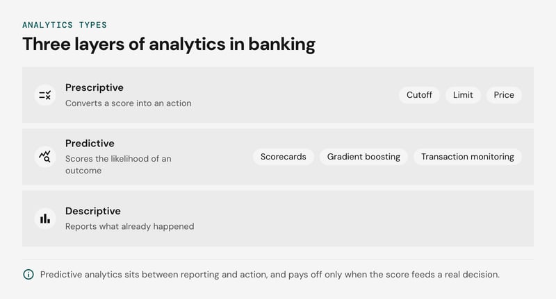
Predictive analytics in fintech works the same way, and it pays off only when the score feeds a real decision.
Descriptive analytics reports what already happened, and prescriptive analytics recommends the action to take. Predictive analytics sits between them and scores the likelihood of an outcome, from logistic regression scorecards in underwriting to transaction monitoring models in fraud and AML.
Netguru builds machine learning, risk and fraud-prevention software and data platforms for financial services and fintech clients. We recommend fixing the decision and its reason-code duty first, because that determines whether a scorecard or gradient boosting is allowed. The constraint loosens for decisions with no explanation duty, such as cash forecasting.
Predictive vs prescriptive analytics in banking
Predictive analytics in banking estimates a probability, and prescriptive analytics converts it into an action through a cutoff, limit or price. A gradient boosting model that outputs a 9% fraud probability or a 4% default probability has predicted, but it has not decided anything.
The policy layer sets the threshold from error costs. Assume a card-fraud model where a wrongly declined payment costs $8 in friction and review, and a missed fraud costs $120 (illustrative assumptions, not benchmarks). Blocking pays off when the fraud probability exceeds 8 / (8 + 120), about 6.3%. AUC ranks cases but does not locate that break-even point. Calibration does.
Treat the policy as its own versioned artifact, separate from the model. Run champion/challenger testing on the cutoff as well as on the model: route a small traffic slice to a challenger threshold and compare realized cost, not offline Gini.
In lending, outcomes exist only for approved applicants, so moving a cutoff into previously declined territory needs reject inference or a controlled test band. Without one, the cost estimate for that region is a guess.
Predictive analytics use cases in banking and the decision each drives
Each predictive analytics use case in banking feeds one specific decision: approve or hold a payment, set a credit limit, pick a retention offer, order a collections queue, or size a funding buffer.
The model output matters only through that decision, so the decision defines the data, the error costs and the risk.
The use cases side by side:
| Use case | Decision it drives | Typical data | Main risk |
|---|---|---|---|
| Transaction monitoring (fraud, AML) | Approve, step up authentication, hold, or route an alert to an analyst | Transaction streams, device and session signals, counterparty links, customer history | Confirmed-outcome labels arrive weeks late, and false positives flood the analyst queue |
| Credit scoring and underwriting | Approve or decline, set limit and price | Bureau tradelines, application data, account history | Selection bias in the approved-only sample; reject inference is an assumption |
| Thin-file scoring | Approve with a low starting limit, or refer to manual review | Bank-account cash flow, payroll deposits, rent and utility payments | Alternative features that proxy for protected classes |
| Churn and next best offer | Who receives a retention offer, and which product | Balances, product holdings, app events, complaints | Targeting customers who would have stayed anyway |
| Collections | Contact order, channel, and forbearance or escalation | Roll rates, payment history, contact outcomes | Self-cure bias in the training population |
| Liquidity and cash forecasting | Funding buffers, ATM replenishment, intraday limits | Inflow and outflow time series, calendar effects | Behavior shifts that break historical patterns |
| Customer lifetime value | Acquisition spend, pricing, service tier | Margin by product, tenure, cross-holding | Long-horizon labels that do not exist for new customers |
Transaction monitoring is the most latency-sensitive row, because the decision happens while the customer waits. Netguru built a risk and fraud prevention solution for a global technology provider to financial services that evaluates risk so accepting or rejecting a transaction is decided automatically, with a dashboard that presents fraudulent transactions so clarification cases are processed quickly. For model design in that setting, see our fraud detection with machine learning guide.
Thin-file customers are the row where the table hides the most work. With little bureau history, a cash-flow model has to be validated on outcomes the bank has rarely observed, and every added feature needs a check for proxy effects before it reaches adverse action reason codes.
A feature store earns its place in the real-time rows. Fraud and thin-file scoring both read features online that were trained on batch history, and a shared feature definition is the usual way to prevent training/serving skew.
The batch rows, such as collections and liquidity forecasting, can often run without one.

How predictive analytics works: Data, features, model, decision
Predictive analytics in banking runs in four steps: build labeled data, compute features, train a model, and wire its score into a monitored decision. Each step has a failure point that offline AUC will not show you.
- Data and labels. Extract transactions, bureau files and servicing history into versioned snapshots, with Apache Airflow scheduling the extraction and validation jobs. Label delay is the constraint. A default label needs a performance window, often a year or longer, so the newest cohorts are unlabeled. Fraud labels arrive only after disputes and chargebacks. Set a window per product, exclude immature cohorts, and use roll rate as an early proxy where the window is too long.
- Features. Define each feature once in a feature store and serve the same definition offline for training and online for scoring. Without one, training runs on batch SQL while serving runs on re-implemented service code. A 30-day rolling count with different window boundaries or null handling is enough to cause training/serving skew. The symptom is production AUC well below validation, and the diagnostic is PSI between training features and logged serving features.
- Model. Gradient boosting usually rank-orders better on tabular fraud, churn and collections data with many interactions. SHAP (Lundberg and Lee, NeurIPS 2017) gives per-decision attributions. Logistic regression scorecards give fixed points per attribute and monotonic, auditable behavior.
We recommend a scorecard as the production model for lending decisions that must produce adverse action reason codes, and as the benchmark any boosted challenger must beat. A constrained boosted model with SHAP-derived reasons can be defended, but expect a longer validation cycle.
Whether it passes depends on your validators and supervisor. MLflow tracks each run and registers model versions alongside the data snapshot and feature set they came from.
- Decision and monitoring. The score becomes a cutoff, a limit, or a queue order. Log every score with the feature values that produced it so any decision can be recomputed later. Run challengers in shadow deployment, track PSI and realized performance as labels mature, and let Airflow trigger the retraining pipeline when drift thresholds trip.
Credit scoring models for thin-file borrowers
Credit scoring for thin-file customers works when alternative data, such as bank-account cash flow, adds signal the bureau file lacks and every adverse decision maps to reasons an applicant can act on.
Unbanked and underbanked households overlap with thin-file customers but are not the same group. The FDIC National Survey of Unbanked and Underbanked Households sizes them: in 2023, 4.2 percent of US households were unbanked and 14.2 percent were underbanked (FDIC National Survey of Unbanked and Underbanked, 2023).
Cash-flow, rent and utility payment data can score applicants a bureau file cannot. Each source needs documented consent and a proxy check for protected classes (see AI bias).
Three failure modes decide whether the scorecard survives model validation:
- Reject inference. Declined applicants have no outcome, and thin-file applicants are declined most often, so a model trained on approvals is biased where you most need it. Parceling or augmentation can partly correct this, but the evidence that it helps is mixed. Validate on approved accounts near the cutoff. A small randomized approval band below the cutoff gives unbiased outcomes where policy and law allow it, and the loss budget for it is a credit-policy decision.
- Label conflicts. An account 90 days past due may cure, while charge-off follows product-specific policy and lags behind. Choose the window with a roll-rate analysis. Keep one definition across training, monitoring and champion/challenger comparisons, because mixed definitions make AUC and KS incomparable.
- Unstable reason codes. SHAP (Lundberg and Lee, NeurIPS 2017) attributes a score to features, and the top negative contributors become the reasons on the ECOA Regulation B adverse action notice. 12 CFR 1002.9 requires specific reasons. CFPB Circular 2022-03 says model complexity is no excuse, and Circular 2023-03 says sample-form reasons must reflect the factors used.
Correlated features swap rank across retrains, so the same applicant can receive different reasons after a model refresh. We recommend grouping correlated features into reason-code families before ranking and fixing the SHAP background dataset. Log reason-rank stability for each retrain in MLflow and treat it as a release gate.
Overfitting hits thin files hardest, because few default events have to support many candidate variables.
Fraud and AML transaction monitoring
Transaction monitoring uses predictive models to score each payment for fraud or money-laundering risk and route it to accept, reject or manual review. Model families are covered in the fraud detection with machine learning deep-dive. The failure modes below decide whether those scores stay useful in production.
Labels are the first problem. Chargebacks confirm card fraud, but they arrive weeks after the transaction, so the most recent training window has the least reliable labels. Validate on a time-based split that excludes the immature window, and treat recent performance as provisional.
Confirmed laundering labels are scarcer, and suspicious activity report filings are a biased proxy because they only record the alerts analysts chose to escalate.
AML adds alert fatigue. A model that raises recall by flooding analysts with alerts lowers real throughput, and analysts start closing alerts by reflex, which contaminates the next round of labels. Track alerts per analyst-hour and the escalation rate next to AUC and KS, and set the threshold against investigation capacity.
Concept drift is faster here than in credit because fraudsters adapt to the controls. Gama et al.'s survey of concept drift adaptation (ACM Computing Surveys, 2014) separates sudden from gradual drift. Watch feature PSI and weekly precision, recall and AUC-ROC so drops surface before they hurt business results. Promote retrained models only after champion/challenger testing in shadow deployment.
Automated declines also raise questions under GDPR Article 22(1), which covers decisions based solely on automated processing that produce legal or similarly significant effects. Legal counsel should confirm whether a blocked payment qualifies in your product.
Churn, next best offer and customer lifetime value
Churn, next best offer and customer lifetime value models pay off when each score triggers a specific action and is monitored for consent and behavior shift after launch.
A churn score ranks who is likely to leave, but it does not say whom a campaign will change; we recommend acting on the score alone when the retention step is cheap and identical for everyone, such as a reminder or a fee waiver.
Once the offer costs margin, move to an uplift model, because a discount sent to a customer who was staying is pure loss. Uplift needs a randomized holdout from past campaigns. Without one, ship the churn score and run champion/challenger testing on the campaign itself.
Consent limits the feature set. Marketing models often draw on behavioral and transaction data whose lawful basis differs from the one covering the account.
Tag each feature in the feature store with its purpose and consent status, and filter on those tags at both training and serving. Where processing rests on consent, Article 13(2)(c) GDPR requires telling customers they can withdraw it at any time.
A withdrawal then has to remove that customer's features from scoring, not only from the CRM.
The GDPR Article 22 threshold applies here too. A reminder email rarely reaches it. An offer that sets price, limit or access to credit may, and legal counsel should confirm where each use case sits.
Offer models decay faster than risk models because the target is behavior that campaigns and rate moves themselves change. This is concept drift. After a rate change, acceptance can fall while PSI on the inputs stays flat. Monitor realized acceptance by score decile against expectation, with a retraining trigger on that gap.
Customer lifetime value extrapolates the same behavior forward. Our view is to use it to rank segments over a short horizon, not as a currency for budget decisions.
Collections, early-warning and liquidity forecasting
Choose roll-rate models for collections queues and time-series forecasts for liquidity; the forecast horizon and the cost of a late action decide between them.
A roll rate is the share of balances that moves from one delinquency bucket to the next. It suits queues where the action is a call or payment plan within days, and a missed cure window is what costs money.
Early-warning on performing accounts has a horizon of months. A logistic regression scorecard on behavior data fits there because its reason codes are easy to validate and explain when a score changes a limit.
Treasury forecasting sets its horizon by funding lead time. If the desk can only source funds a day ahead, forecast daily and use calendar features such as payroll and tax dates. A late action costs spot borrowing or an idle buffer, so judge accuracy in currency terms.
The trade-offs side by side:
| Use case | Horizon | Model | Cost of a late action |
|---|---|---|---|
| Collections queue | Days to one billing cycle | Roll-rate model | Lost cure window |
| Early-warning default | Months | Logistic regression scorecard | Limit or provisioning set too late |
| Liquidity forecast | Intraday to weeks | Time-series with calendar features | Spot funding or idle buffer |
All three degrade through concept drift. Rate changes and hardship programs alter how accounts roll. Track population stability on bucket transitions and forecast error against actuals. Apache Airflow can run daily scoring, error checks and retraining as dependent tasks, so a drift alert blocks promotion of a stale model.
Regulation that shapes model design: EU AI Act, GDPR, Regulation B and SR 11-7
Model design in banking is shaped by the EU AI Act, GDPR Article 22, US adverse action rules and SR 11-7 model risk management. Each fixes a design choice: how the model is documented, who can override a score, and how a decline is worded.
The rules side by side:
| Rule | What it requires | Design consequence |
|---|---|---|
| EU AI Act, Regulation (EU) 2024/1689 | Annex III lists creditworthiness assessment of natural persons as high-risk. Most of the Regulation applies from 2 August 2026, but the Digital Omnibus on AI, Regulation (EU) 2026/1744, deferred Annex III high-risk obligations to 2 December 2027. | Write Annex IV technical documentation during development: design assumptions, validation data, accuracy metrics, tests for discriminatory impact, human oversight measures. |
| GDPR Article 22 and the CJEU SCHUFA ruling (C-634/21) | Article 22(1) gives the right not to be subject to a solely automated decision with legal or similarly significant effects. Article 22(3) requires human intervention, the chance to state a view, and the right to contest. In C-634/21, the Court treated a credit agency's probability score as an automated decision where the lender draws strongly on it. | Send declines and marginal score bands to reviewers who can override. Log each override and its reason. Treat bought-in bureau scores as in scope. |
| Regulation B, 12 CFR 1002.9 and CFPB Circular 2022-03 | An adverse action notice must state the specific reasons for the decision. The Circular says a creditor cannot cite the complexity of an algorithm as a reason it cannot do so. | Generate reason codes from per-decision attributions such as SHAP. Check that they name features that drove the score, and version them with the model. |
| SR 11-7 (mirrored by OCC Bulletin 2011-12) | Documented development, independent validation, ongoing monitoring and effective challenge, backed by a model inventory. | Keep a simple benchmark, such as a logistic scorecard, next to every gradient-boosted challenger. Record the lift that justifies the added complexity. |
Supervisors also expect the choice of a complex model to be explained. The scorecard benchmark gives you that explanation as a measured gap, which a validator can challenge.
Bias testing needs protected attributes. Article 4a of the AI Act, added by Regulation (EU) 2026/1744, allows providers of high-risk systems to process special categories of personal data for bias detection only when strictly necessary and when synthetic or anonymised data cannot do the job.
It also requires access controls and deletion once the bias is corrected. Plan an isolated store for those attributes, kept out of the feature store.
SR 11-7 and the OCC bulletin are supervisory guidance, not statute, and Regulation B applies to US creditors only. Which of these rules binds you depends on where you lend and to whom, so have counsel confirm scope and the dates that apply to your products.
Why predictive models fail in fintech, and the fix for each
Predictive models in fintech fail from thin or biased data, inconsistent labels, overfitting, concept drift and explainability gaps, and each failure has a fix with a metric and a trigger.
The failures side by side. The PSI trigger is a common rule of thumb, not a regulatory threshold:
| Failure | Fix | Metric | Trigger |
|---|---|---|---|
| Thin or biased data | Reject inference, segment-level validation | Gini and approval rate per segment | Segment gap above the tolerance your model risk team sets |
| Inconsistent labels | One versioned default definition, such as a fixed delinquency window | Label agreement across sources, roll rate | Any definition change forces revalidation |
| Overfitting | Feature pruning, out-of-time validation | Train versus out-of-time Gini and KS | Gap widens between releases |
| Concept drift | DDM or ECDD on the error stream, PSI on inputs | PSI per feature, score-band stability | PSI above 0.25 on a top feature starts retraining |
| Explainability gap | SHAP reason codes mapped to decline wording | Stability of top-ranked reasons | A reason with no plain-language mapping blocks release |
Biased data is the failure that reaches regulators first. Check performance by segment before launch, and treat AI bias as a validation item, not a post-launch audit. Labels need the same discipline: if collections and risk define "default" differently, the model learns the disagreement.
Overfitting is usually a feature-count problem: too many candidate variables for too few events. Prune features, then score the pruned model on an out-of-time sample, not a random holdout.
Concept drift is the slow failure. DDM and ECDD (an exponentially weighted moving average detector) watch the error stream and signal drift, which replaces manual periodic checks. Wire the signal to an Apache Airflow retraining job. Log every run in the MLflow Model Registry so each score traces to a model version.
On explainability, SHAP gives per-decision attributions that can feed adverse action reasons. In Germany, the Bundesbank and BaFin list explainability among their supervisory expectations for machine learning in risk models. Keep a simpler benchmark model so the gain from a complex one is measured, not asserted.
A retrained model should never replace the production scorer directly. Run it in shadow mode first, then in champion/challenger testing on a slice of live traffic, and promote only after validation sign-off under SR 11-7 model risk management. We recommend recording the promotion criteria before the test starts, so the result cannot be argued after the fact.
Tools for predictive analytics in banking
Choose predictive analytics tooling for banking by three deployment constraints: batch or real-time scoring, audit trail, and lineage. No single tool is best across all three.
The mapping we recommend:
| Constraint | Tool | What it covers |
|---|---|---|
| Batch scoring (collections, churn, liquidity forecasts) | Apache Airflow | Schedules feature and scoring jobs with dependencies, retries and a run history |
| Real-time scoring (fraud, card and payment decisions) | Feature store with online serving | One feature definition for training and serving, which limits training/serving skew |
| Audit trail and model inventory | MLflow | Tracks experiments and versions models in a registry, so each production model traces to its parameters and metrics |
These tools do not overlap. Airflow orchestrates jobs but does not version models, and MLflow records models but does not schedule retraining.
Stack fit decides the rest. If your cloud already offers managed equivalents and your validators accept them, use those before adding self-hosted components.
Before the first model goes live, check that the build covers six items, each mapped to the documentation and validation expectations in SR 11-7 and OCC Bulletin 2011-12:
- Versioned data snapshots with lineage from source to feature.
- One label definition, recorded with its performance window.
- Drift thresholds per top feature, with a named owner for each alert.
- A retraining pipeline that cannot promote a model on its own.
- Champion/challenger testing with promotion criteria written before the test.
- Human review for declines and marginal score bands, with every override logged.
FAQ
What are the three main types of predictive analytics?
What are five common predictive analytics models in banking?
Which tool is best for predictive analytics in banking?
Plan a predictive analytics build with Netguru
Planning predictive analytics in banking starts with three fixed points: the decision the model drives, the label definition, and the named owner who signs off under SR 11-7 model risk management.
We recommend a short discovery that settles those, plus explainability and drift-monitoring requirements, before any modeling begins. Our overview of data science in finance covers the wider context, and our financial services work shows the products we build for banks and fintechs.
If you want a second opinion on scope, data readiness or validation design, bring the decision, the data sources and your constraints, and we will help you add AI to your product.


